Possible Principle of Controlling the
Self-Assembly of Biomolecular Materials
This is a draft paper
for a talk at the
Fifth
Foresight Conference on Molecular Nanotechnology.
The final version has been submitted
for publication in the special Conference issue of Nanotechnology.
This page uses the HTML <sup> and
<sub> conventions for superscripts and subscripts. If
"103" looks the same as "103"
then your browser does not support superscripts. If "xi"
looks the same as "xi" then your browser does not
support subscripts. Failure to support superscripts or
subscripts can lead to confusion in the following text,
particularly in interpreting exponents.
Abstract
One reports computational study aimed at possible principle
of controlling the biomolecular self-assembly whose course may be specified by
features characterizing changes in the patterns of expanding spatial regions in
which molecular components exhibit appearance of required properties. Diversity
in ways of the expansion influenced by stochastic factors is simulated by
appropriate random process constituted of a number of independent (parallel)
realizations of covering nodes of the hexagonal grid. For modelling the
finite-size effects resulting from contribution of supramolecular structures to
the expansion, the information about covering a node is transmitted: between
members of a pair of neighbour nodes and due to conditional displacement of
this pair (actually, information about organization of two nodes into a pair is
displaced between grid nodes). The state at each stage is represented by the
pattern constructed so that it is as close as possible, after situation in
space and measure, to all the various sets being the process state realizations
at this stage; this is mean measure set (MMS). The MMS evolution pattern
enables us to pursue features of generating the collective effect resulting
from the process realizations. We have parametrized conditions in which two
subsequent rapid strong increments in the MMS area covered exhibit qualitative
change in form, from sedimentation-like increment to percolation-like one (the
events are separated by the resident time). We discuss conditions for using the
process parameter to control appearance of the qualitative change and try to
suggest actual methods which would be used to control the self-assembly
corresponding to the simulations.
1. Introduction
Biomolecular materials and structures are those whose
molecular-level properties are abstracted from biology and are structured or
processed in a way that is characteristic of biological materials, but they are
not necessarily of biological origin (NAS 1996). A key feature of biomolecular
materials is their ability to undergo self-assembly that is coordinated action
of independent objects or entities under influence of factors that are not
centralized; this action leads to formation of structures with required
properties. The self-assembly is one of strategies used in biology for the
development of complex, functional structures and can incorporate them directly
as components in the final systems which can be relatively defect-free and
self-healing (Whitesides 1991,1995). One complex system of living Nature and
the other belonging to unanimated world of mechanics have inspired us to
suggest a class of biomolecular materials and structures whose self-assembly
would be controlled by appropriate change in the ambient conditions of the
process.
1.1 Two inspiring examples
A natural example appears to be provided by the
ensemble composed of thousands of blood platelets experiencing independently
transformations just after their adhesion to an artificial surface. The
platelets are then situated on the surface within a single layer and spread in
close proximity one to another. In those conditions, redistribution of certain
transmembrane proteins on the flow side of the platelets' membranes results in
collective effect that is facilitating the anchorage of the self-assembling
fibrin net, forming the second platelet layer and thus further initiation of
the thrombus. Displacements of the transmembrane proteins are associated with
the platelet cytoskeleton remodeling (Mosher 1993, Smith et al 1992) and,
indirectly, with membrane skeleton remodeling (Behnke and Bray 1988). Groups of
the proteins tethered (even temporarily) by the cytoskeleton fragments (Sixma
et al 1989) may contribute to the collective effect of the transmembrane
proteins redistribution. The collective effect generation mechanism can be
investigated using a model that requires considering the displacements of not
tethered proteins or groups of tethered transmembrane proteins as point objects
or finite-size entities, respectively. Displacements of the finite-size
entities and the point objects associated with their origination contribute to
the collective effect. Manifestations of this contribution represented in
certain averaged description of the protein redistribution and referred to all
platelets of the ensemble are identified as an example of finite-size effects.
This representation at each stage of the platelet ensemble evolution may be
realized by constructing a single pattern being as close as possible to all the
patterns representing the transmembrane protein redistribution on membranes of
all the platelets of the ensemble at the stage. The sequence of those single
patterns corresponding to subsequent stages of the platelet ensemble evolution
would be employed to pursue the collective effect generation.
The example from the world of mechanics is
given by turbulent wall-bounded flow. Results of previous research on turbulent
transport (Kozlowski 1996) have suggested that features of the collective
effect generation may be controlled by appropriate change in ambient conditions
of the process for systems exhibiting the finite-size effects. They have shown
that appearance of the finite-size effects in a complex system admits regime in
which the system may appear in either of the alternative states in ambient
conditions unchanged. These conditions have been parametrized and it has
appeared that the regime may occur only for certain intervals of the control
parameter. Change in the conditions, specified by change in value of the
control parameter such that it exits the interval mentioned implies jump in
averaged values of the structural characteristic of the system state which
indicates switch to the unambiguous regime. Values of the structural
characteristics specifying the new state of the system differ from those
specifying state of the system on the other side of the control parameter
interval. Those structural characteristics represent average, collective effect
of action of an ensemble of various complex finite-size organized fluid
entities contributing to transport processes within the system. It has been
found that neglecting the finite-size effects in the simulations of the system
behavior implies absence of the characteristic features associated with change
in value of the control parameter. This has suggested that features of
collective effect generation may be controlled by appropriate change of ambient
conditions for systems exhibiting the finite-size effects. On the other hand,
direct influence on phenomena contributing to the finite-size effects would be
a way of controlling the self-assembly of the biomolecular materials
also.
1.2 A class of materials considered
Association of the revealed opportunity with the natural
example has inspired us to distinguish a class of the biomolecular materials
self-assembling from systems specified by the following features assumed:
- They are composed in a form of the ensemble of many complex
subsystems of the same kind (but they are not the same) that experience
independently transformations under influence of stochastic factors in the same
ambient conditions. Composition of the initial system (a molecular medium with
suspended nanostructures or other ingredients) would permit for originating of
a large number (incomparable, however, to the Avogadro number) of the
subsystems that will further develop due to various chemical reactions.
- The course of transformations of each complex subsystem can
be specified by features characterizing changes in the pattern of expanding
spatial regions in which certain components of the subsystem exhibit appearance
of required properties.
- Transformations of all the subsystems can result in a
collective effect generated by whole the ensemble. Appearance of the collective
effect can indicate finish or a discrete step in the self-assembling.
- Expansion within each subsystem or within the vast majority
of the subsystems can be considered of as resulting also from contribution of
certain finite-size structures able to transmit information portion by
themselves (between their ends) and due to effective finite displacement of
those structures. Manifestations of this contribution which are represented in
certain averaged description of the whole system transformation are identified
as finite-size effects.
This class encompasses wide spectrum of biomolecular
materials and structures including the future biomolecular membranes being much
simpler than natural cell membranes and performing their selected functions
(e.g. NAS 1996). The finite-size effects would result from synthesis and action
of mechanically-interlocked molecules (like those reported by Amabilino and
Stoddart (1995) which would contribute to the expansion process. On the other
hand, extraordinary properties of carbon nanotubes pointed out by Globus (1997)
make them attractive component of biomolecular materials or structures
exhibiting finite-size effects in course of their self-assembly. It is worth
considering also the opportunity for application of the self-replicating
positional devices ,like assemblers proposed by Merkle (1996), for forcing
occurrence of these effects under programmatic control. The self-assembly on
surfaces seems to be here good candidate for performing the control in the way
of changing the ambient conditions of the process: Actually there are known
examples were self-assembly is function of temperature (MM 1996) ; there are
also grounds for believe that encouraging the self-assembling material
formation in particular regions of the surface may be possible in the way of
the proper surface modifications (Goddard et al 1996).
The revealed opportunities would be used to control the
self-assembly by varying certain parameters specifying ambient conditions of
the process. Candidates for those parameters may be suggested basing on results
of appropriately parametrized computer simulations of a model complex system
possessing features of the real systems alluded to previously. In this paper we
propose that simulation , parametrize it and perform variant computations
revealing role of the particular parameters in the collective effect
generation. This enables us to make certain suggestions concerning actual
methods which would be used to control the self-assembly corresponding to the
simulations.
2. Simulation: assumptions and method
The expansion of spatial regions in which molecular
components exhibit appearance of certain required properties can be simulated
of as resulting from an appropriately constructed process of information
transmission in course of covering certain spatial domain assumed. Diversity in
ways of the expansion realization influenced by stochastic factors is simulated
by random expansion process (REP) whose states at subsequent stages of its
development are finite random sets (FRS) being set multiplicity of realizations
that have evolved independently (in parallel) within the same spatial domain.
The state at each stage is represented by the pattern constructed so that it is
as close as possible, after measure and situation in space , to all the various
realizations at the stage. This is mean measure set (MMS) characterizing mean
expected form of the REP and it is determined accordingly to method proposed by
Vorobiev (1984). Results of the study on mechanisms contributing to appearance
of changes in the MMS features will provide representative information on
generation of the collective effect corresponding to final stage or an
intermediate discrete step of the self-assembly. Let us note , herein, that
sets constituting the multiplicity FRS are not necessarily to correspond , one
to one, to the complex subsystems of the real system simulated ; a number of
these sets is to be only as large as to provide opportunity for adequate
representation of the diversity in expansion realizations for the complex
subsystems. This number is to be established specifically for a particular
process simulated. That manifestation of the finite-size effects by the complex
system appears to provide opportunity for controlling the collective effect
generation by changing ambient conditions has resulted from previous study
(Kozlowski 1996) where application of discrete space for simulations enabled us
to model the finite-size effects appropriately. In virtue of this result, the
space with discrete topology (this is not Zariski space) has been chosen here
for the simulations. Reference to the natural systems expanding on a surface
implies specification of the discrete space so that its elements coincide with
nodes of a regular grid on a plane.
We use the space S
={xi , i=1,2,...,Ns} whose finite number of Ns
points are nodes of the regular hexagonal grid (here, we apply
Ns=145x124 so that the grid covers the square 1x1). Each node is
center of the regular hexagon that filled with certain color illustrates
inclusion of the node to the subset of the S which is identified by this
color. This grid has largest density of nodes among all the grids for which the
same value of the smallest distance between the nodes is given (Hilbert and
Cohn-Vossen 1932). For a discrete space (generally , for compact spaces) , a
feature peculiar to each node which specifies situation of all its nearest
neighbours is characteristic for whole the space as well (Janich 1984) . This
implies superimposition of the form of a regular hexagon on the patterns
resulting from processes of covering the nodes in course of simulating the
expansion on the grid. It has appeared possible to avoid this effect in the way
of specific randomization of distribution of realizations of the grid nodes'
vicinities composed of such nodes being nearest neighbours of each node which
are admitted for covering. Eventually, the local feature of the grid structural
regularity has not been copied to local rules of covering the nodes ( rationale
of this method will have been presented elsewhere). Normal covering is
hereafter referred to the case for which all nearest neighbours of each node
can be potentially covered due to signal transmission from the node surrounded.
The term randomized covering indicates that choice which subset of a node
nearest vicinity could be potentially covered due to signal transmission from
the node surrounded has been done randomly for each node of the grid. Each of
the two space covering specifications performed prior to the simulation could
be referred to respective limit form of a prepatterned surface at which the
self-assembly corresponding to the simulation might be realized. Therefore we
report here results obtained with both the specifications.
We have incorporated the idea of discrete
displacements employed to model the finite-size effects for certain example
of complex systems (Kozlowski 1996) into the simplest variant of the Markov
process proposed for modeling random displacements (Vorobiev 1984). In result
we have obtained the modified version of the Markov process of independent
realizations. State of this REP at a stage IT is given by a finite number
NK of its realizations Ai accomplished independently one
from another . This state is denoted as KIT ={Ai ,
i=1,2,...,NK}. With the purpose to sketch the way of constructing
the KIT+1 from the KIT we note series of
neighbourhoods Gz , Gzz with: node 'z' being element of
the Ai at stage IT for each 'i' (i.e. the 'z' is also the element of
KIT) ; node 'zz' being an element of the neighbourhood
Gz ,and Hz being set-theoretical union of the
neighbourhoods Gzz for all elements 'zz' of the Gz. This
enables us to construct a vector HK such that each of the
NK its elements indicated by index i=1,2,..., NK is
set-theoretical union composed of sets Hz for all elements 'z' of
the realization Ai at the stage IT. For each i=1,2,...,NK
, realization (Ai)IT+1 of the KIT+1 is
constructed as set-theoretical union of sets (Rx)i
resulting from local expansions for all nodes 'x' belonging to respective
element with index 'i' of the vector HK. Explanation of the
(Rx)i requires presentation of a set
{(Ai)IT.and.Gy} being common part of the set
(Ai)IT and the neighbourhood Gy of the node
'y' being element of the neighbourhood Gx of the node 'x' in respect
to which the (Rx)i is accomplished. For each element 'y'
of the Gx, replacement of covering of each node 'xx' from the set
{(Ai)IT.and.Gy} with covering of such node
'yy' from the neighbourhood Gxx of the 'xx' that the 'yy' is
situated in respect to 'xx' as the 'y' is situated in respect to the node 'x'
results in set of the nodes 'yy' which may constitute the
(Rx)i. The transmission of information about organization
of two nodes into a pair , (x,y).to.(xx,yy) identified as effective
transposition of the pair (x,y) complements information portion about covering
of a node which can be transmitted by the pair between its nodes , (x.to.y) or
(xx.to.yy) . This is the way in which the finite size effects alluded to
previously are modelled within frame of the REP. In virtue of the explanations
given above for the Hz , the 'x' is an element of the Gzz
and, generally, the situation y=x is valid also. The node 'yy' is covered ,
i.e. it is an element of the (Rx)i when certain
probability Py(x) assigned for the simulation to a node 'y', being
an element of the seven node vicinity ( SNV) of the node 'x', is not less than
a random value f(y,i). The 'f' is generated , specifically for the 'y' and REP
realization number 'i' , as an element of the random vector obtained with the
help of available random number generator RANMAR (James 1990). The values
Py(x) are elements of the vector of seven probabilities ( VSP)
assigned to the hexagon of seven nodes with the 'x' in its center (i.e. to the
SNV of the 'x' ). Here, it has been assumed that VSP is the same for all the
nodes of the grid (a sum of the seven probabilities of the VSP is within the
interval (0,1]).
Eventually, the REP is simulated as Markov process of covering nodes
of a regular hexagonal grid and so that information about covering a node
is transmitted : between members of a pair of neighbour nodes and due to
conditional displacement of this pair. Displacement of information about
organization of two nodes into a pair identifies the effective displacement
of the pair of neighbour nodes. This may be considered as generalization
of the discrete displacement method (DDM) developed previously (Kozlowski
1996) for modelling similar finite-size effects peculiar to turbulent transport
and verified for example of the developed turbulent pipe flow.
Let us recall that computed realizations Ai ,
i=1,2,...,NK of the K are employed here to simulate specific
diversity in the process realizations whose mean expected form is characterized
by the mean measure sets at each stage IT. They are closest after their
situation and measure to all the various realizations Ai at the
stage considered . This multiplicity has unique , single set representation at
the stage; this is also called mean measure set - MMS and has been determined
using the method proposed by Vorobiev (1984). One searches also for the set of
nodes covered in each realization Ai of the K ; this set
denoted as ker(K) is called core of the K. One finds also a set
of nodes covered at least in one realization of the K ; this set denoted
as bas(K) is called base of the K. These characteristics can be
found at each stage IT of the REP. Vanishing of the core for each IT>1 has
appeared to be convenient criterion of establishing the sufficiently large
value NK for the REP simulated here (we have found
NK=100).
3. Results and discussion
We have searched for conditions of the expansion
simulation which would result in the sequence of the MMS patterns with
features revealing qualitative change in the MMS increment associated with
jumps in value of the countable measure Imms of the MMS (just
, number of nodes of the MMS). Tentative computations have suggested observing
that situation after breaking symmetry of the expansion in the space. Therefore
, for focusing attention just on the phenomenon searched for we have constructed
the vector of seven probabilities (VSP) admitting expansion in one halfplane
only. This has been done by specifying the VSP by a single parameter
P25:=P2=P3
=P4 =P5 with P7= 0 and
P1=P6
= 0 . The scheme
                               P2
                         P1=0        P3
                               P7=0
                         P6=0        P4
                               P5
of the VSP and its parametrization with the P25 , the same
for all nodes of the S , fill in the requirement. Here, the value
P7= 0 assumed excludes the possibility of coincidence of the
node 'y' with 'x' and thus only pairs of neighbour nodes contribute to
the expansion. Moreover, one admits only two possible instances of
displacements
of the pairs: In the first instance, no node of the pair displaced can
occupy position of any node of the pair before the displacement (i.e. 'xx'
can coincide neither with 'x' nor with 'y'). Lack of the displacement
corresponds
to the second instance (then 'xx' coincides with 'x' whereas 'yy' coincides
with 'y'). Accordingly, it has been assumed that node 'zz' cannot coincide
with the node 'z' ,and node 'x' cannot coincide with the node 'zz'. The
process has been started from two straight separated chains of covered
nodes to improve reliability of the results. Their vertical situation has
been chosen in accordance with the VSP scheme. They are assigned to IT=0
so that
bas(K0)=ker(K0)=MMS(K0)
, although the physical start occurs at IT=1 from the K1
represented by the MMS(K1) whose pattern has a form of
the two chains of small islands. We have constrained number of the time
steps of the REP simulations with the purpose either to avoid superimposition
of part of the bas(KIT) developing from one chain onto
this expanding from the second one or to prevent the bas(KIT)
from approaching the boundary of the area assigned to the S.
The research performed for randomized space covering
specification has revealed an interval of the parameter,
0.1<P25<0.17
for which simulation of the REP results in a series of few jumps in increment
of the MMS measure Imms preceded and followed by resident times
with very weak specific variation of the Imms (see
figure 1 [b/w] ). We have assigned
numbers IA to subsequent stages at which the jumps occur so that
IT(IA+1)>IT(IA)+1
and the resident time defined as number of stages that separates the subsequent
jumps is expressed by equation, t(IA)=IT(IA)-IT(IA-1) with IA>0. Observation
of two dimensional MMS patterns specified by the jumps in Imms
has enabled us to find the first one
{MMS(KIA)\MMS(KIA-1)}
exhibiting the qualitative difference from the previous MMS increments
(the backslash denotes the set-theoretical difference, e.g. for sets A,
B : {A\B}={A.without.[elements of B]}). Then nodes constituting the increment
{MMS(KIA)\MMS(KIA-1)} appear to be
distributed throughout the MMS(KIA-1) , contrary to previous
cases where area of the MMS increment resulting from the jump is just stuck
to right of the MMS pattern preceding this jump. This qualitative change
resembles switch from sedimentation-like form of the increment to
percolation-like
one. Appearance of this first specific jump in Imms can be observed
for the second residence time t(IA=2) ; see figure 1
[b/w] and sequence of the patterns
{MMS(KIA)\MMS(KIA-1)}
depicted in series starting with figure 2 to figure 7
[b/w] that have been obtained for P25=0.16.
For analysing the organization process that may be recognized
in the sequence of the MMS patterns we have constructed the entropy
characteristic
H. To this aim the notion of set theoretical ruler with length Sn
has been proposed and the notion of gliding hexagon - GH has been used.
The GH consists of seven nodes coinciding with the grid nodes so that a
node indicating location of the GH is surrounded by its six nearest neighbours.
The Sn is equal to the number of such locations of the GH within
the smallest rectangle enveloping the bas(KIT) that for
each of these locations there is a fixed number 'n' of nodes covered
constituting
a single chain within the GH (the 'n' is not less than 2 and not more than
7). Let the number of possible locations of the GH within that rectangle
be denoted by MGH . One may consider increment in informative
entropy of finding a sample node covered - SNC within the domain MGH
which results from appearance of the SNC within single chains of 'n' covered
nodes at the Sn locations of the GH. This value is denoted as
Hn for the one number 'n' fixed whereas H identifies this value
for all the 'n' being elements of the set {2,3,4,5,6,7}. That the SNC may
appear within the chain just mentioned affords the opportunity for using
the ruler Sn to find the SNC within the domain MGH
with the probability Sn/MGH. The values Sn
are determined elementary and the characteristics referred to the information
entropy are expressed accordingly to general formulae known:
the H is expressed as a sum of Hn after n=2 to 7 with Hn=
-( Sn/MGH)ln(Sn/MGH).
The characteristics just expressed are denoted as Hmms or
(Hn)mms
, respectively when they are determined for the MMS. Mathematical expectations
Hav or (Hn)av of the H or Hn
determined for all the realizations Ai , i=1,2,...,NK
of the K have been presented here for comparison with these referred
to the MMS. Alternations of the Imms within the 't' correspond
to variation of the MMS pattern and its reference to bas(K) that
can be seen in distribution of the Hmms against IT (see
figure 8 [b/w] ). The Hmms
diminishes for the residence time preceding the jump in the Imms.
This jump is accompanied by the one in the Hmms to the
Hmms
local maximum from which this value diminishes for the residence time preceding
the subsequent jump. Here, first act of the MMS increment, whose pattern
shows the new features alluded to previously, is preceded by the residence
time t(IA=2) extending just to left of the stage IT=IT(IA=2)=42 at which
both the values Hmms and Hav are maximal. Additional
simulations performed without regard to the finite size effects have not
permitted for selecting conditions in which the patterns of the MMS increments
show that feature.
Results for the normal space covering specification
are depicted in figures 9 , 10 [b/w]
(characteristics) and figures 11
, 12 [b/w] (MMS increments). They have been obtained
for simplified version of the REP , for which the HK
is replaced by the KIT i.e. node 'x' is taken as element
of the KIT only (see section 2 for references). We have
simulated this version of the REP also for the randomized space covering
specification and found that the qualitative change in the MMS increment
can be observed for the control parameter interval,
0.18<P25<0.23.
On the other hand, applying the normal space covering specification results
in reduction of that interval to the one extending less than 0.001 on both
sides of the P25=0.104. Then, however, the switch in the form
of the MMS increment is more distinct than for simulation with the randomized
space covering specification. This seems to suggest that an intermediate
space covering specification, between utterly randomized and the normal
one, would afford opportunity for controlling features of the qualitative
change in the MMS increment when supremum of the Hmms is achieved.
We were not able to achieve the qualitative change in the MMS increment
for the symmetric expansion i.e. with the VSP such that PJ=P/6
with 0 < P < 1 for each J=1,2,...,6 ; those simulations were started
either from chains of nodes or sets constituting filled rectangles situated
in few ways in the space. This seems to suggest that asymmetry in local
expansion may be the necessary condition here. The simulations performed
with the VSP realizing this condition in several ways suggest that , for
the aim pursued, the VSP should not prefer a single direction (i.e. only
one of the six for this grid) to strongly but be close to the VSP used
for simulations reported in this paper.
4.Conclusions and suggestions
The results analysed seem to reveal potential opportunity for controlling
generation of the collective effect resulting from the biomolecular
self-assembly
for a class of the systems considered here (see Section
1.2). This would be done by changing ambient conditions of the process.
Realizing of the control would require imposition of a factor resulting
in spatial asymmetry of the two-dimensional expansion , the same for all
the expanding complex subsystems constituting the relevant real system
in which self-assembly takes place. This might be done e.g. by an acoustic
action, imposed shear, an electric field with an appropriate characteristic
or concentration gradient of a chemical component in the initial environment.
Application of those factors should be associated with properties peculiar
to the self-assembling material or structure with the purpose to realize
the asymmetry condition in the way corresponding to this used for the
simulations
reported (see section 3). Parameter specifying the
asymmetry resulting from the particular value of that factor would correspond
(qualitatively) to the parameter P25 . On the other hand , degree
of ordering of the prepatterned surface on which the self-assembly is realized
would correspond to an intermediate space covering specification in the
simulation reported (see section 2 and 3). Then, selecting
the value of the imposed factor together with the degree of ordering of
the prepatterned surface would make possible controlling features of the
collective effect resulting from various realizations of the expansion
in all the complex subsystems of the ensemble constituting the system.
Comparison of the results obtained from simulation performed at normal
and randomized space covering specification suggests that required selection
of a value of the factor being imposed may appear to be hardly possible
for the perfectly ordered prepatterned surface (then the acceptable value
might be found within very short interval only). That qualitative change
in form of the MMS increment is observed at supremum of the Hmms
in course of the expansion simulated may suggest single occurrence of the
corresponding event in the relevant real system.
The noted role of the finite-size effects makes worth considering the
opportunity for forcing occurrence of these effects under programmatic
control in particular regions of the surface.
Acknowledgments
Major part of the computations has been performed by using
computational facilities in Institute of Biophysics and Biochemistry ,
PAS , Warsaw, Poland. A part of the results has been obtained by using
resources of the Interdisciplinary Centre for Mathematical and Computational
Modelling at Warsaw University, Poland.
References
- Amabilino D B and Stoddart J F 1995 Interlocked and
Interwined
Structures and Superstructures, Chem. Revs. 95 2725-828 See
also http://www.che.bham.ac.uk/Research_labs/Research_Profiles/jfstoddart/self-ass.html
http://www.che.bham.ac.uk/Research_labs/Research_Profiles/jfstoddart/stoddart_res03.html
- Behnke O and Bray D 1988 Surface Movements During Spreading
of Blood Platelets, European Journal of Cell Biology 46 207-16
- Globus A , Bauschlicher C , Han J , Jaffe R , Levit C
and Srivastava D 1997 Machine Phase Fullerene Nanotechnology , paper at
Fifth Foresight Conference on Molecular Nanotechnology 5-8 November 1997,
Palo Alto , California , http://www.foresight.org/Conferences/MNT05/Nano5.html
see also: http://science.nas.nasa.gov/Groups/Nanotechnology/publications/1997/fullereneNanotechnology
- Goddard III W A , Cagin T and Walch S P 1996 Atomistic
Design and Simulations of Nanoscale Machines and Assembly , NASA sponsored
project report , http://www.wag.caltech.edu/gallery/nano_comp.html
- Hilbert D and Cohn-Vossen S 1932 Anschauliche
Geometrie
(Berlin) in German
- James F 1990 A Review of Pseudorandom Number Generators,
Computer Physics Communications 60 329-44
- Janich K 1984 Topology (New York Berlin Heidelberg
Tokyo : Springer-Verlag)
- Kozlowski W 1996 A Method of Discrete Displacements for
Modeling the Contribution of Finite-Size Organized Fluid Structures to
Transport Processes in Turbulent Pipe Flow, International Journal for
Numerical Methods in Fluids 23 105-24
- Merkle R C 1996 Design Considerations for an Assembler,
Nanotechnology 7 210-5 See also http://nano.xerox.com/nanotech/nano4/merklePaper.html
- Mosher D F 1993 Adhesive Proteins and Their Cellular
Receptors, Cardiovascular Pathology 2(3) S149-55
- Smith C M, Burris S M, Rao G H R and White J G 1992
Detergent-Resistant
Cytoskeleton of the Surface-Activated Platelet Differs from the Suspension
Activated Platelet Cytoskeleton, Blood 80(11) 2774-80
- Sixma J J, Van den Berg A and Hartwig J 1989 Immunoelectron
Microscopic Localization of Actin, Alpha-Actinin, Actin Binding Protein
and Myosin in Resting and Activated Human Blood Platelets, European
Journal of Cell Biology 48 271-81
- Vorobiev O Yu 1984 Mean Measure Modelling (Moscow
: Nauka) in Russian
- Whitesides G M, Mathias J P and Seto C P 1991 Molecular
Self-Assembly and Nanochemistry: A Chemical Strategy for Synthesis of
Nanostructures,
Science 254 1312-9
- Whitesides G M 1995 Self-Assembling Materials, Scientific
American 273(3) 114-7 See also http://nano.xerox.com/nanotech/nano4/whitesidesAbstract.html
- MM 1996 Self-Assembled Monolayers and Electron-Beam Resists
, Materials Matter (PENNSTATE PA : Materials Research Institute)
1(2) 13- 4,16 , see also: http://www.mri.psu.edu/programs/newsltr/content2.html
- NAS 1996 Biomolecular Self-Assembling Materials
(Washington DC : National Academy Press) http://www.nas.edu/bpa/reports/bmm/bmm.html
to figures presented in black/white or
gray-scale
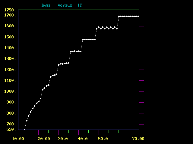
Figure 1. Evolution of the MMS measure,
P25=0.16 ; random
space covering specification [b/w] (see
section 3)
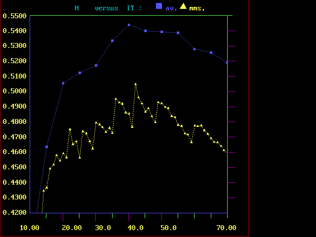 \ \
Figure 8. Evolution of the entropic characteristics,
P25=0.16
; random space covering specification [b/w] (see
section 3)
(to figures representing results with
normal space covering specification [b/w]
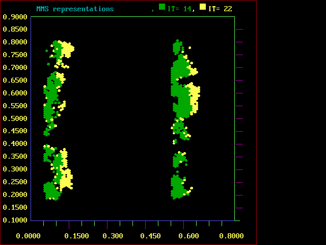
Figure 2. MMS increment (indicated by yellow color in
Figures 2 to 7), P25=0.16
[b/w] (see section 3) ;
Figures 2 to 7 represent results obtained
with random space covering specification ; scroll to compare
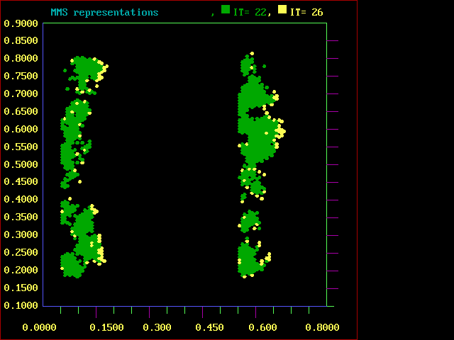
Figure 3. MMS increment,
P25=0.16
[b/w]
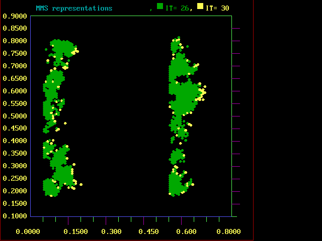
Figure 4. MMS increment ,
P25=0.16
[b/w]

Figure 5. MMS increment from IA=0
to IA=1 , P25=0.16
[b/w] (see
section3 for
explanations)
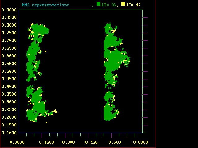
Figure 6. MMS increment from IA=1
to IA=2 , P25=0.16
[b/w] (see
section 3 for
explanations)
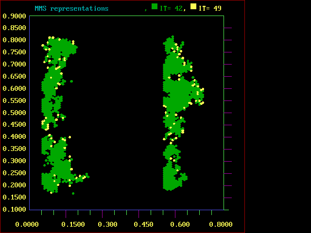
Figure 7. MMS increment from IA=2 to IA=3 ,
P25=0.16
[b/w] (see
section 3 for explanations)
(to Figure
8
[b/w]
back
to Figure 1) [b/w]
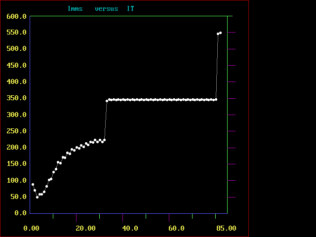
Figure 9 Evolution of the MMS measure
, P25=0.104 ; normal
space covering specification [b/w]
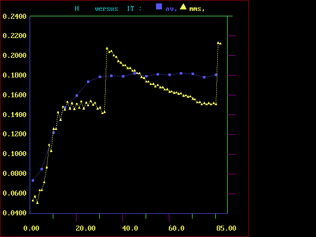
Figure 10. Evolution of the entropic characteristics ,
P25=0.104 ; normal
space covering specification [b/w] (see
section 3)
(to figures representing results
obtained with random space covering
specification
)[b/w]
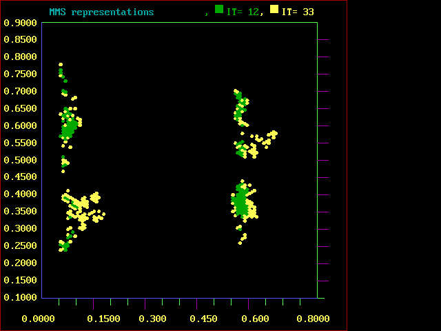
Figure 11. MMS increment from IA=0 to IA=1 (indicated
by yellow color in figures 11 and 12), P25=0.104
; [b/w]
patterns depicted in figures 11 and
12 have been obtained with normal space covering specification
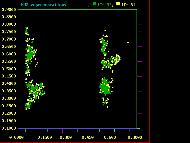
Figure 12. MMS increment from IA=1 to IA=2 ,
P25=0.104
; normal space covering specification [b/w] (see
section 3)
(to figures representing results for random
space covering specification )
to figures presented in
colors
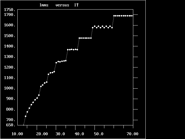
Figure 1. Evolution of the MMS measure,
P25=0.16 ; random
space covering specification [cr] (see
section 3)
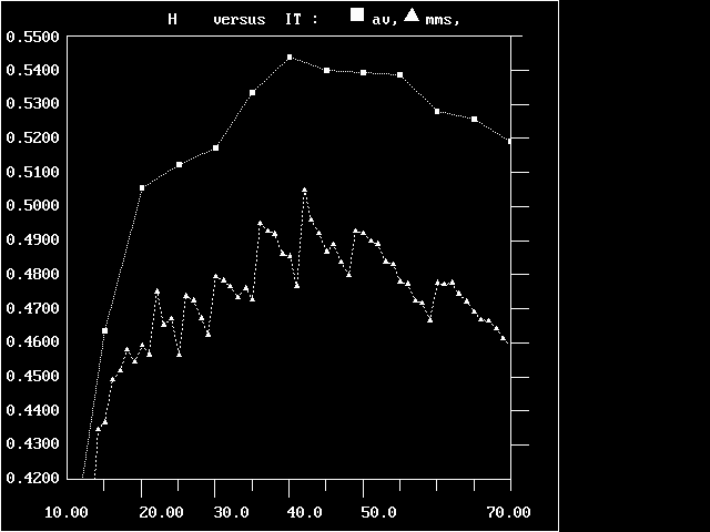 \ \
Figure 8. Evolution of the entropic characteristics,
P25=0.16
; random space covering specification [cr] (see
section 3)
(to figures representing results with
normal space covering specification [cr]
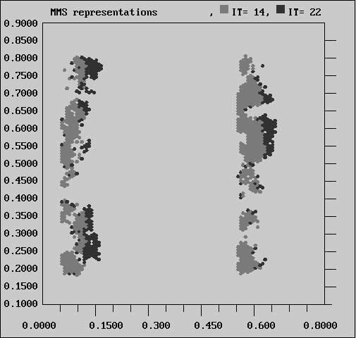
Figure 2. MMS increment (indicated by yellow color in
figures 2 to 7), P25=0.16
[cr] (see section 3) ;
Figures 2 to 7 represent results obtained
with random space covering specification ; scroll to compare
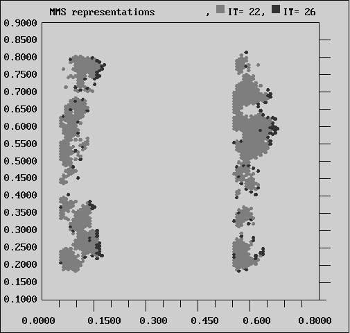
Figure 3. MMS increment, P25=0.16
[cr]
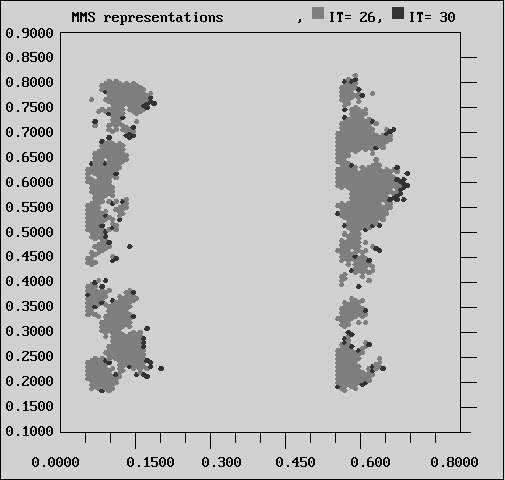
Figure 4. MMS increment ,
P25=0.16
[cr]
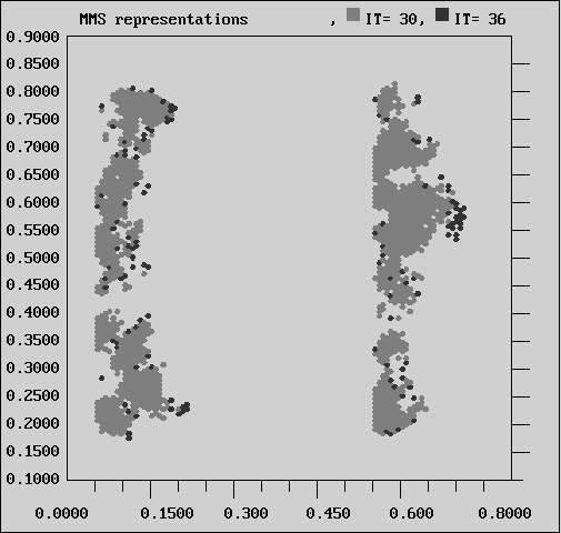
Figure 5. MMS increment from IA=0 to
IA=1 , P25=0.16 [cr]
(see section3
for explanations)
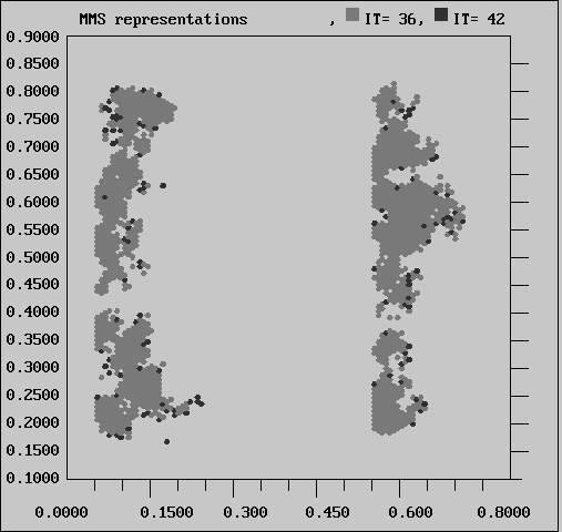
Figure 6. MMS increment from IA=1 to
IA=2 , P25=0.16 [cr]
(see section 3
for explanations)
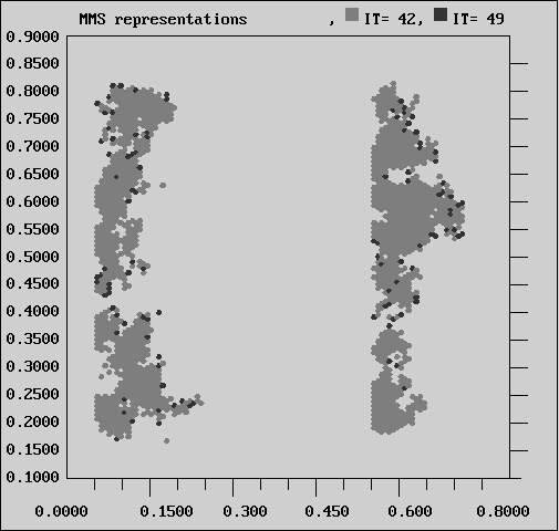
Figure 7. MMS increment from IA=2 to IA=3 , P25=0.16
[cr] (see
section 3 for explanations)
(to Figure
8
[cr]
back
to Figure 1 [cr])
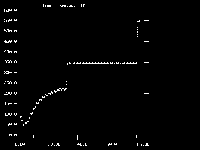
Figure 9 Evolution of the MMS measure
, P25=0.104 ; normal
space covering specification [cr]
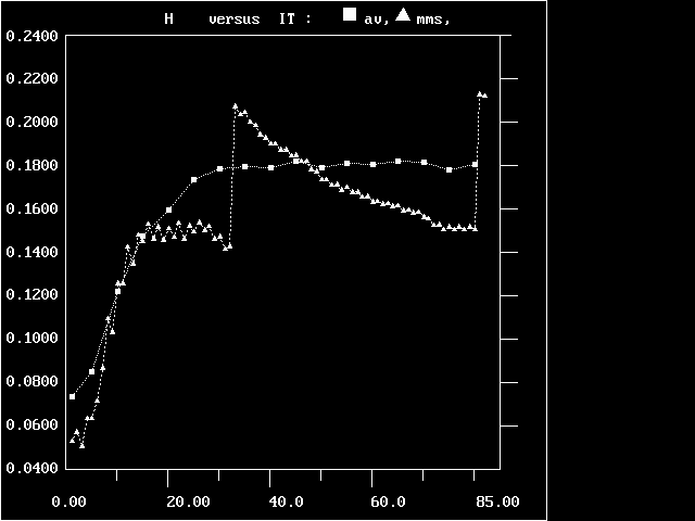
Figure 10. Evolution of the entropic characteristics ,
P25=0.104 ; normal
space covering specification [cr] (see
section 3)
(to figures representing results obtained
with random space covering specification
[cr]
)
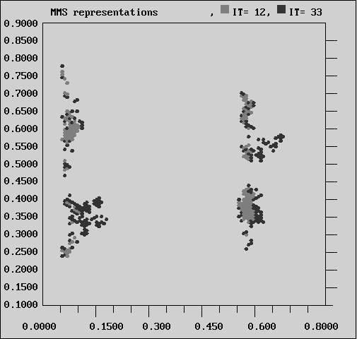
Figure 11. MMS increment from IA=0 to IA=1 (indicated
in black in Figures 11 and 12), P25=0.104
; [cr]
patterns depicted in Figures 11 and
12 have been obtained with normal space covering specification
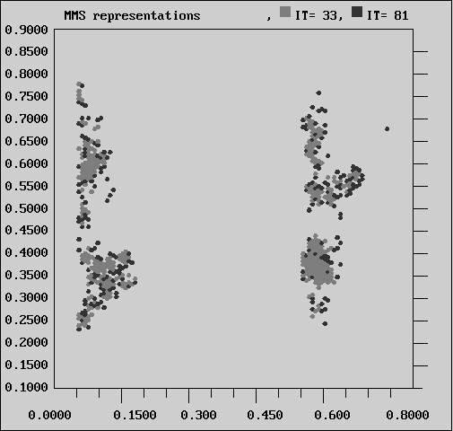
Figure 12. MMS increment from IA=1 to IA=2 ,
P25=0.104
; normal space covering specification [cr] (see
section 3)
(to figures representing results for random
space covering specification ) [cr]
|